Technical reference
1) The method to seek Lyapunov exponents
The calculation by Wolf's algorithm leads the Lyapunov exponents from the reconstructed attractor made by
time series data. The method of Wolf shows on Figure 14.
Figure 14
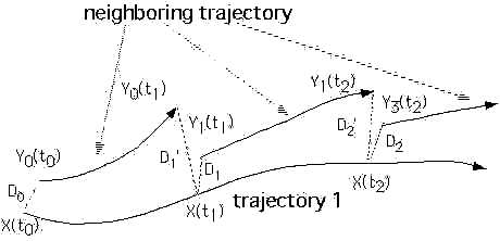
Note the point X (t0) and the trajectory Y0, and Y0 (t0) is
the nearest trajectory neighboring by original trajectory one. After the decided time passed, X (t0) moves to X (t1)
and Y0 (t0) moves to Y0 (t1). On the point X (t1) the new trajectory Y1 (t1) is chosen by the condition of the most
neighboring and the same direction of the trajectory of one step before, and Y1 (t2) is selected after the decided time passed. The choice of the nearest trajectory by this method is done on the total trajectory one. Distant D0 changes to distance D1, so Distant Dj changes to distance Dj+1, and D2/D1 or Dj+1/Dj is the rate of the expansion of each coordinate. Because log (Dj+1/Dj)/(tj+1-tj) exhibits an exponential expansion of attractor from one coordinate,
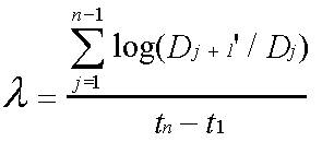 -- (1)
shows Lyapunov exponents that are the average of the exponential expansion of total attractor from each coordinate. By these methods Lyapunov exponents are calculated from the reconstructed attractor made
by time series data from the histopathloogical image of skin diseases.
2) The method to seek correlation dimension
The calculation of correlation integral on the reconstructed attractor leads correlation
dimension that is a kind of fractal dimension. Correlation dimension is derived from the correlation
integral defined by
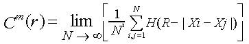 --- (2)
H(y) is the Heaviside function (1 if y >=O and O if y < O).
Xi ( i = 1, 2,・・・・, N) are the points on the reconstructed attractor of
m dimensional space. We count the number of point Xj (j=1, 2,・・・・, N; i not j) within
a ball made in the m dimension with a center of Xi and with a diameter of r.
The summation of the count of Xj within a ball by all Xi leads the correlation integral.
If the correlation integral is scaled in the suitable range of r, the correlation exponent v (m) is defined as
Cm(r) ∝ rv(m) -- (3) ( m is the dimension of the reconstructed dimension).
Therefore, if the formula 3 is confirmed in the reconstructed attractor in any range
of r (for example r1 <r < r2), the self resemblance will be admitted
in r1 <1 r < r2. V(m) is the ratio of logCm(r) vs log r between the suitable
log r ranges. The true correlation dimension of phenomenon is unknown, if the examined data
is derived from the experimentation or the real physical phenomenon. When the dimension m
is smaller than the real attractor dimension, the attractor will fulfill the reconstructive
space and v(m) will be equal to m (m is called embedding dimension in this process).
Thus the v (m) increases as the increase of the dimension m, and finally reaches a certain
value that will indicate correlation dimension.
This conversion of v (m) means the existence of the self-resemblance that is one of
the characteristics of chaos, and if no conversion is observed, the possibility of the existent
of chaos is low. The high value of the correlation dimension assumes to show high
complexity or multiple deviation of the original phenomenon. Xi coincides
with Yj in the calculation of this study. The dimensional parameter m coincides with n.
3) Dynamical system
The dynamical system of n dimension is presented as follows;
Xt+1 =F( Xt , u ), Xt ∈ Rn
Xt : A state of a system in t
F( ) : mapping of n dimension
u : parameter vectors of a system.
t: discrete time
We can observe the stable state in n dimensional system, and the stable state is
called attractor of the discrete dynamical system. Attractor converges to three states of
fixed points, periodic attractor and strange attractor by changing u. It is strange attractor
that chaos shows on its trajectory in dynamical system. Chaos has the properties of orbital
instability, long-term unpredictability and self-similarity. Although there are many parameters
to prove the existence of chaos, Lapyanov exponents and correction dimension are effective
characteristics.
Lyapunov exponents (demonstrate the orbital instability)
In n dimensional dynamic space as Xt+1 =F( Xt , u ), Xt ∈ Rn, if
a ball which shows the primary status and has a diameter of a is
changed to the next status of an oval ball by one mapping,
Xt changed to Xt+1 by function F( ), and λ1 ,λ2 ・・・λn shows
the exponential magnifying or diminishing rate of each direction.
The value ofλ1 ,λ2 ・・・λn are called Lyapunov exponents, and
at least one positive Lyapunov exponent shows the inability of long
term prediction of chaos. Correlation dimension demonstrates
the self-similarity of attractor in dynamical system.